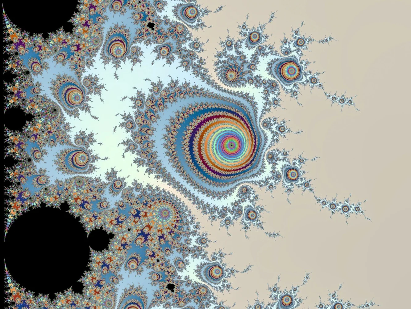
Introduction: storing a rule instead of pixels
A digital image usually looks like a huge table of values. Compression represents that table with fewer bits.
JPEG transforms blocks into frequencies and quantizes the coefficients. Other codecs use prediction, wavelets, larger transforms, context models or neural networks.
Fractal compression asks a different question. Can one region be reconstructed from another after scaling, rotation, reflection, contrast change and brightness shift?
Instead of storing the pixels of a target block, the encoder stores an instruction: "Take this larger region, reduce it, rotate it, adjust contrast and brightness, and place it here." A complete image can be described by many such transformations.
The decoder repeatedly executes them. After several iterations, the image stabilizes. The compressed representation behaves like a small program whose output is a fixed point.
How can an image be reconstructed from pieces that do not yet exist at the start of decoding? The fixed-point theorem provides the answer.
An image does not need to be fractal. The practical method exploits approximate local similarities. It does not assume perfect self-similarity of the entire photograph.
An image as a point in a space
A W by H grayscale image can be viewed as a vector with WH components. A distance between images may be based on mean squared error:
A transformation W maps one complete image to another: . The decoder seeks a fixed point X* such that W(X*) = X*. The code stores W rather than directly storing X*.
The code stores an operator. The decoder does not read the final image. It applies a rule whose reconstructed image is the fixed point.
Contraction and the fixed-point theorem
W is contractive if there is an s with 0 ≤ s < 1 such that:
Banach's fixed-point theorem guarantees a unique fixed point, convergence from every initial image, and an error that decreases geometrically. After n iterations:
If s = 0.5, after ten iterations the maximum gap is divided by about 1,024. If s is close to 1, convergence is much slower.
Contractivity is the guarantee. Without a factor less than 1 in the appropriate metric, the existence and uniqueness of the result are no longer guaranteed.
IFS: a few transformations, one attractor
An IFS contains contractive maps , …, . The Hutchinson operator is: [1]
Repeated application converges to an invariant attractor A such that W(A) = A. The Barnsley fern is a famous example. A handful of affine transformations produces a complex shape. The chaos game applies a probabilistically chosen transformation to a point. After a transient, the points draw the fern.
This demonstrates that a short rule set can generate rich geometry. A natural photograph, however, is not an exact global IFS attractor.
[[figure:IFSExplorer]]
The collage theorem: solving the inverse problem
Compression solves the inverse problem. Given a target image X, find W whose fixed point X* is close to X. If W has contraction factor s and d(X, W(X)) ≤ ε, then:
The encoder therefore seeks an operator that leaves the target almost unchanged. The theorem is a bound, not an automatic optimal encoder.
Why a photograph is not a perfect fern
Photographs contain textures, shadows, perspective, edges, noise and unique details. Their self-similarity is partial and local. A region may resemble another only after downsampling, rotation, reflection, contrast scaling and brightness shifting.
Jacquin's practical block coding exploits piecewise self-transformability rather than exact global fractality.
From IFS to PIFS
Partitioned IFS coding divides the image into non-overlapping range blocks. For every range block , the encoder searches a larger domain block . After downsampling, geometry and photometric adjustment: [2]
A code stores: domain position, symmetry, contrast factor, brightness offset, block size, partition information. All codes together define the global decoder operator.
Range and domain blocks
A 512 by 512 image may use 8 by 8 range blocks and 16 by 16 domains. The domain is reduced to the range size. The larger domain provides cross-scale redundancy and helps spatial contractivity.
For every range, a brute-force encoder may test thousands of domains and eight symmetries. That search dominates runtime.
[[figure:BlockMatcher]]
Geometric transformations
A square block commonly uses eight symmetries:
- Identity
- Rotation 90°
- Rotation 180°
- Rotation 270°
- Horizontal reflection
- Vertical reflection
- Diagonal reflection
- Anti-diagonal reflection
More flexible methods may use general affine mappings or irregular partitions. Flexibility improves approximation but increases search and code size.
Contrast and brightness
The photometric mapping is:
where s changes contrast and o changes brightness. Contractive coding typically restricts |s| < 1.
If s = 1 and o = 0, intensities are preserved. If s = 0, the block produces a uniform region equal to o. Values must also be quantized and clamped.
Fitting a transformation by least squares
For domain values and range values , minimize:
The optimum is:
Uniform domains require robust special handling. The chosen s is clamped to the contractive range before error evaluation.
The encoding algorithm
For every range block: enumerate candidate domains, downsample each domain, test symmetries, fit s and o, compute error, keep the best code.
Encoding searches, decoding executes. This asymmetry explains both the elegance of the decoder and the historical cost of the encoder.
Why encoding is expensive
The complexity is roughly:
Decoding applies known transformations. Encoding must discover them. Acceleration methods include block classification, variance and moment signatures, smaller domain pools, nearest-neighbor search, k-d trees, vector quantization, quadtrees, approximate search, GPU parallelism.
Quadtree and adaptive partitioning
A fixed partition wastes bits in simple regions and undersamples complex ones. A quadtree begins with large ranges. If the approximation error is too high, split the block into four.
Lower thresholds create more blocks, higher bitrate and better fidelity. Higher thresholds create smaller files with larger error. The partition itself must also be encoded.
[[figure:QuadtreeExplorer]]
The decoding algorithm
The decoder may start from black, white, noise or any arbitrary image. For every code: read its domain from , downsample, apply symmetry, apply s and o, write the range into . Then .
Two buffers should be used so one iteration does not depend on write order.
[[figure:FractalDecoder]]
Why the initial image barely matters
For two initial images and :
Their difference vanishes geometrically. After enough iterations, both produce essentially the same decoded image. The stable information is in the transformations, not in the starting pixels.
Convergence speed and contraction factor
To reach tolerance τ:
A contraction of 0.5 converges quickly. A contraction near 0.9 may require many more iterations. A noncontractive case should be demonstrated only as a failure mode outside the codec guarantee.
Measuring distortion: MSE, PSNR, SSIM and bitrate
Mean squared error:
For 8-bit images:
SSIM compares local luminance, contrast and structure. Bitrate is bpp = compressed bits / pixel count. Fair comparison requires rate–distortion curves under one protocol. No single quality number tells the whole perceptual story.
A good image does not prove a good codec. Bitrate, distortion, time, memory and protocol must be compared across multiple images.
Typical artifacts
- Repeated textures
- Softened edges
- Synthetic-looking detail
- Block boundaries
- Flattened areas
- Contrast errors
- Substituted unique features
- Painted or artificial appearance
Texture-rich and repetitive regions may work well. Fine text, faces, symbols and unique details are harder.
Fractal zoom: promise and limit
The transformation code can be evaluated on a finer grid. This creates scale-consistent interpolation. It does not recover missing truth. The new details are generated by the model. They may be plausible but not authentic.
Fractal zoom must never be treated as forensic or medical detail recovery. The details are generated, not recovered.
JPEG versus fractal compression
JPEG stores quantized transform coefficients. Fractal coding stores relations between image regions and decodes iteratively.
JPEG benefits from fast encoding, standardization and hardware support. Fractal coding offers a generative fixed-point interpretation and strong encoder–decoder asymmetry. Neither method is universally superior.
Why the method did not dominate
- Expensive encoding
- Variable image-dependent quality
- Difficult rate control
- Strong competition from standards
- Proprietary and patent history
- Exaggerated historical claims
The method remains scientifically valuable because it frames compression as inverse modeling.
Contributions to computer science
Fractal compression illustrates:
- An image as a program
- Fixed-point decoding
- Nonlocal prediction
- Cross-scale redundancy
- Multiresolution representation
- Nearest-neighbor optimization
- The overlap between modeling and compression
Relation to modern generative representations
There is a conceptual resemblance between fractal codes and modern implicit or learned representations. Both store parameters and execute a decoder. The mechanisms differ. A classical PIFS uses explicit transformations and contractivity. A neural representation learns a function by optimization and need not be contractive or interpretable.
This is an analogy, not an automatic historical lineage.
Where is the spiral?
Fractal compression is mainly about convergence, not visible spirals. A rotating contraction:
with |a| < 1. The distance to the fixed point decreases as |a|ⁿ while the angle increases by θ. The trajectory forms a discrete spiral.
Image decoding follows a trajectory in a very high-dimensional space. That trajectory is not necessarily a geometric spiral. The shared structure is contraction plus convergence.
Convergence, not obligatory spiral. The fixed point is central. A spiral trajectory only appears if the contraction also includes a rotational component.
Conclusion
Fractal compression replaces a storage problem with a generation problem. It asks which transformations have an image as an approximate fixed point.
The encoder searches for self-transformations. The decoder iterates them. Contractivity removes the initial state. The fixed point appears.
The method did not become the dominant general-purpose codec, but it remains one of the clearest demonstrations that data can be represented as a dynamical system rather than a list of values.
References
- [1]Barnsley, Michael F.. (1988). Fractals Everywhere. Academic Press
- [2]Jacquin, Arnaud E.. (1992). Image Coding Based on a Fractal Theory of Iterated Contractive Image Transformations. IEEE Transactions on Image Processing, 1(1), p. 18–30. DOI: 10.1109/83.128028. https://pubmed.ncbi.nlm.nih.gov/18296137/