1. Introduction
Economies do not grow in a straight line. They experience expansions, slowdowns, crises and recoveries. These fluctuations have very different durations: a few months for an inventory cycle, a few years for a classic business cycle, several decades for what some economists call long waves. The Kondratiev hypothesis belongs to this last category.
This article presents the hypothesis honestly: its origins, proposed mechanisms, proponents and critics. It emphasizes the considerable methodological difficulties that prevent it from being validated or refuted with certainty. It distinguishes what is established, what is plausible and what belongs to metaphor.
2. Nikolai Kondratiev and His Data
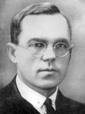
Nikolai Dmitrievich Kondratiev (1892–1938) was a Soviet economist who directed the Moscow Institute of Conjuncture. In his work of the 1920s, he analyzed price, production and interest rate series for several industrialized countries — primarily England, France and the United States — over periods roughly from 1780 to 1920. He identified oscillations of approximately 40 to 60 years in these series.
The data used by Kondratiev were limited by current standards. Historical price and production series from the 19th century are fragmentary, often reconstructed after the fact, and their quality varies considerably. Kondratiev himself acknowledged that his observations covered only two to two-and-a-half cycles, which is insufficient to establish a statistically robust periodicity.
Kondratiev was arrested in 1930 during the Stalinist purges, convicted for allegedly predicting the survival of capitalism, and executed in 1938. His work was rediscovered in the West in the 1970s, when stagflation and oil shocks seemed to confirm the idea of a long-term turning point.
3. Technological Waves: Schumpeter and His Successors
Joseph Schumpeter gave a technological interpretation to Kondratiev waves in his work Business Cycles (1939). He associated each wave with a cluster of major innovations: the first wave (1780–1840) with the steam engine and textiles; the second (1840–1890) with railways and steel; the third (1890–1940) with electricity, chemistry and automobiles; the fourth (1940–1990) with petrochemicals and electronics.
Later authors proposed a fifth wave linked to information and communication technologies (approximately 1990–2040), and some already speak of a sixth wave linked to biotechnology, renewable energy and artificial intelligence. These proposals are appealing but circular: a dominant innovation is identified after the fact and associated with a period of growth.
Carlota Perez developed a more sophisticated version of this theory in Technological Revolutions and Financial Capital (2002). She distinguishes two phases in each technological revolution: an installation phase (with a financial bubble) and a deployment phase (with productive diffusion). This analysis is more nuanced than the simple innovation-growth association, but remains difficult to test quantitatively.
4. Proposed Mechanisms
Several mechanisms have been proposed to explain long waves. The fixed capital investment mechanism assumes that major infrastructures — railways, electrical grids, highways — have lifespans of several decades. Their construction creates intense demand, then their depreciation frees resources for new investments. This investment cycle could generate long-duration oscillations.
The credit and debt mechanism assumes that expansions are financed by credit expansion, which creates financial imbalances. Correcting these imbalances takes time and can depress the economy for a decade or more. Hyman Minsky developed a theory of financial instability that shares some elements with this view, without necessarily postulating a fixed periodicity.
The institutional mechanism assumes that each technological revolution requires institutional adaptations — new regulations, new educational systems, new forms of work organization — that take time to establish. The transition period between technological deployment and institutional adaptation would be a source of economic turbulence.
These mechanisms are individually plausible, but their combination and interaction are difficult to model. No formal model has succeeded in deriving a 40–60 year periodicity from economic first principles without assuming ad hoc parameters.
5. Why the Hypothesis Is Difficult to Test
The first difficulty is the limited number of observable cycles. If waves last 40–60 years, available data since the industrial revolution cover only three to four complete cycles. This is insufficient to distinguish a real periodicity from coincidence or statistical artifact. In statistics, it is generally considered that at least 20–30 cycles are needed to establish a periodicity with reasonable statistical power.
The second difficulty is the non-stationarity of economic series. Economies change in structure, size and technology over time. A wheat price series from the 19th century is not directly comparable to an industrial production index from the 20th century. Statistical methods that assume stationarity — such as classical spectral analysis — can produce misleading results on non-stationary series.
The third difficulty is the choice of dates. The peaks and troughs of waves are often defined after observation, choosing the points that best fit the theory. This ex post selection bias is difficult to avoid and can create the illusion of periodicity where there is none. A robust theory should specify in advance the indicators, the tolerated duration and the falsification criteria.
The fourth difficulty is the multiplicity of structural breaks. The two world wars, the Great Depression, decolonization, the end of the Bretton Woods system, oil shocks, globalization and the digital revolution have all profoundly altered the structure of economies. These breaks make episodes difficult to compare and complicate the identification of regular cycles.
6. The Statistical Debate
Statistical studies on Kondratiev waves have produced contradictory results. Some spectral analyses have found significant peaks around 50 years in price or production series. Other studies have shown that these peaks disappear when different filtering methods, different series or different periods are used. The robustness of the results is low.
Filtering of time series is a major source of ambiguity. Trend-cycle decomposition methods can introduce artificial oscillations whose period depends on the filter parameters. A Hodrick-Prescott filter with a high smoothing parameter can create long-duration cycles that do not exist in the raw data. This criticism was formulated by Cogley and Nason (1995) for business cycles, and it applies a fortiori to Kondratiev cycles.
**Experimental method.** One way to test the hypothesis would be to specify a priori: (1) the economic indicators to use, (2) the expected cycle duration with explicit tolerance, (3) the statistical method, (4) the rejection criteria. Then apply this procedure to data independent of those that inspired the theory. To date, no study has satisfied all of these criteria.
7. Competing Approaches
Classic business cycles, lasting 3–8 years, are better documented and better understood than long waves. They are associated with fluctuations in investment, inventories and consumer demand. DSGE (Dynamic Stochastic General Equilibrium) models can reproduce some of their characteristics, although their realism remains debated.
Financial cycles, lasting 15–20 years, have been documented by the Bank for International Settlements. They reflect expansions and contractions of credit and real estate prices. Their link with business cycles is well established: recessions following a financial expansion are generally deeper and longer.
The exogenous shock theory assumes that economic fluctuations are primarily caused by unpredictable disturbances — technological shocks, oil shocks, financial crises, pandemics — rather than by regular endogenous cycles. In this perspective, Kondratiev waves would be an illusion created by the coincidence of several major shocks.
8. The Spiral as Metaphor for Economic Time
Representing Kondratiev waves on a spiral is a powerful visual metaphor. It expresses the idea that the economy never returns to exactly the same point: each cycle occurs at a different level of technological and institutional development. The spiral captures this combination of repetition and progression.
This metaphor is useful for communication, but must not be confused with proof. A spiral in an economic graph is a representation chosen by the author, not a mathematical property of the data. The same succession of cycles could be represented as a wavy line, a table or a bar chart, without any of these representations being more true than the others.
It is important to distinguish four levels of claim: a statistically demonstrated periodicity (the strongest level, not achieved for Kondratiev); an interpreted historical succession (episodes that resemble cycles, but without precise periodicity); a wave metaphor (a way of speaking about long-duration fluctuations); a spiral representation of time (a visual image without its own empirical content).
9. Scientific Caution
The Kondratiev hypothesis is neither proven nor refuted. It raises a legitimate question — do technological and institutional transformations create long-duration rhythms in economies? — but available data do not allow it to be answered with certainty. This uncertainty must be communicated clearly.
Abusive uses of the hypothesis are numerous. Consultants and forecasters use it to predict economic turning points with a precision not justified by the data. Investors use it to justify long-term strategies based on an undemonstrated periodicity. These uses must be distinguished from serious academic research.
The enduring interest of Kondratiev lies in the question he posed, not the answer he proposed. Understanding how major technological transformations diffuse through the economy, how they interact with institutions and credit, and why some periods seem more dynamic than others: these are important questions that deserve rigorous research, with data, models and honesty about limitations.
Starting with an observed series: GDP levels
Before looking for a long wave, define the measurement. The series below is United States real GDP, published by the Bureau of Economic Analysis and distributed through FRED as GDPC1. Observations are quarterly, in billions of chained 2017 dollars, seasonally adjusted at an annual rate. A point is neither personal income nor the total received during that quarter alone. “Real” indicates a price adjustment; it does not mean that the estimate is immune to revisions. [1]
This snapshot contains 318 observations from 1947 Q1 to 2026 Q2, retrieved on 19 October 2026. It shows long-run growth and changes in slope. Joining the points improves readability but adds no observations between quarters. The scale is linear: an equal absolute change occupies equal height at every date. Comparing proportional changes requires a different representation and an explicit statement of that choice; undulations in levels should not automatically be treated as independent cycles.
Read all 318 observations and download the data
BEA / FRED · GDPC1 · Billions of chained 2017 dollars, seasonally adjusted annual rate.
JSON data — snapshot from 19 October 2026| Quarter starting | Real GDP (billions 2017 $) |
|---|---|
| 1947-01-01 | 2182.681 |
| 1947-04-01 | 2176.892 |
| 1947-07-01 | 2172.432 |
| 1947-10-01 | 2206.452 |
| 1948-01-01 | 2239.682 |
| 1948-04-01 | 2276.690 |
| 1948-07-01 | 2289.770 |
| 1948-10-01 | 2292.364 |
| 1949-01-01 | 2260.807 |
| 1949-04-01 | 2253.128 |
| 1949-07-01 | 2276.424 |
| 1949-10-01 | 2257.352 |
| 1950-01-01 | 2346.104 |
| 1950-04-01 | 2417.682 |
| 1950-07-01 | 2511.127 |
| 1950-10-01 | 2559.214 |
| 1951-01-01 | 2593.967 |
| 1951-04-01 | 2638.898 |
| 1951-07-01 | 2693.259 |
| 1951-10-01 | 2699.156 |
| 1952-01-01 | 2727.954 |
| 1952-04-01 | 2733.800 |
| 1952-07-01 | 2753.517 |
| 1952-10-01 | 2843.941 |
| 1953-01-01 | 2896.811 |
| 1953-04-01 | 2919.206 |
| 1953-07-01 | 2902.785 |
| 1953-10-01 | 2858.845 |
| 1954-01-01 | 2845.192 |
| 1954-04-01 | 2848.305 |
| 1954-07-01 | 2880.482 |
| 1954-10-01 | 2936.852 |
| 1955-01-01 | 3020.746 |
| 1955-04-01 | 3069.910 |
| 1955-07-01 | 3111.379 |
| 1955-10-01 | 3130.068 |
| 1956-01-01 | 3117.922 |
| 1956-04-01 | 3143.694 |
| 1956-07-01 | 3140.874 |
| 1956-10-01 | 3192.570 |
| 1957-01-01 | 3213.011 |
| 1957-04-01 | 3205.970 |
| 1957-07-01 | 3237.386 |
| 1957-10-01 | 3203.894 |
| 1958-01-01 | 3120.724 |
| 1958-04-01 | 3141.224 |
| 1958-07-01 | 3213.884 |
| 1958-10-01 | 3289.032 |
| 1959-01-01 | 3352.129 |
| 1959-04-01 | 3427.667 |
| 1959-07-01 | 3430.057 |
| 1959-10-01 | 3439.832 |
| 1960-01-01 | 3517.181 |
| 1960-04-01 | 3498.246 |
| 1960-07-01 | 3515.385 |
| 1960-10-01 | 3470.278 |
| 1961-01-01 | 3493.703 |
| 1961-04-01 | 3553.021 |
| 1961-07-01 | 3621.252 |
| 1961-10-01 | 3692.289 |
| 1962-01-01 | 3758.147 |
| 1962-04-01 | 3792.149 |
| 1962-07-01 | 3838.776 |
| 1962-10-01 | 3851.421 |
| 1963-01-01 | 3893.482 |
| 1963-04-01 | 3937.183 |
| 1963-07-01 | 4023.755 |
| 1963-10-01 | 4050.147 |
| 1964-01-01 | 4135.553 |
| 1964-04-01 | 4180.592 |
| 1964-07-01 | 4245.918 |
| 1964-10-01 | 4259.046 |
| 1965-01-01 | 4362.111 |
| 1965-04-01 | 4417.225 |
| 1965-07-01 | 4515.427 |
| 1965-10-01 | 4619.458 |
| 1966-01-01 | 4731.888 |
| 1966-04-01 | 4748.046 |
| 1966-07-01 | 4788.254 |
| 1966-10-01 | 4827.537 |
| 1967-01-01 | 4870.299 |
| 1967-04-01 | 4873.287 |
| 1967-07-01 | 4919.392 |
| 1967-10-01 | 4956.477 |
| 1968-01-01 | 5057.553 |
| 1968-04-01 | 5142.033 |
| 1968-07-01 | 5181.859 |
| 1968-10-01 | 5202.212 |
| 1969-01-01 | 5283.597 |
| 1969-04-01 | 5299.625 |
| 1969-07-01 | 5334.600 |
| 1969-10-01 | 5308.556 |
| 1970-01-01 | 5300.652 |
| 1970-04-01 | 5308.164 |
| 1970-07-01 | 5357.077 |
| 1970-10-01 | 5299.672 |
| 1971-01-01 | 5443.619 |
| 1971-04-01 | 5473.059 |
| 1971-07-01 | 5518.072 |
| 1971-10-01 | 5531.032 |
| 1972-01-01 | 5632.649 |
| 1972-04-01 | 5760.470 |
| 1972-07-01 | 5814.854 |
| 1972-10-01 | 5912.220 |
| 1973-01-01 | 6058.544 |
| 1973-04-01 | 6124.506 |
| 1973-07-01 | 6092.301 |
| 1973-10-01 | 6150.131 |
| 1974-01-01 | 6097.258 |
| 1974-04-01 | 6111.751 |
| 1974-07-01 | 6053.978 |
| 1974-10-01 | 6030.464 |
| 1975-01-01 | 5957.035 |
| 1975-04-01 | 5999.610 |
| 1975-07-01 | 6102.326 |
| 1975-10-01 | 6184.530 |
| 1976-01-01 | 6323.649 |
| 1976-04-01 | 6370.025 |
| 1976-07-01 | 6404.895 |
| 1976-10-01 | 6451.177 |
| 1977-01-01 | 6527.703 |
| 1977-04-01 | 6654.466 |
| 1977-07-01 | 6774.457 |
| 1977-10-01 | 6774.592 |
| 1978-01-01 | 6796.260 |
| 1978-04-01 | 7058.920 |
| 1978-07-01 | 7129.915 |
| 1978-10-01 | 7225.750 |
| 1979-01-01 | 7238.727 |
| 1979-04-01 | 7246.454 |
| 1979-07-01 | 7300.281 |
| 1979-10-01 | 7318.535 |
| 1980-01-01 | 7341.557 |
| 1980-04-01 | 7190.289 |
| 1980-07-01 | 7181.743 |
| 1980-10-01 | 7315.677 |
| 1981-01-01 | 7459.022 |
| 1981-04-01 | 7403.745 |
| 1981-07-01 | 7492.405 |
| 1981-10-01 | 7410.768 |
| 1982-01-01 | 7295.631 |
| 1982-04-01 | 7328.912 |
| 1982-07-01 | 7300.896 |
| 1982-10-01 | 7303.817 |
| 1983-01-01 | 7400.066 |
| 1983-04-01 | 7568.456 |
| 1983-07-01 | 7719.746 |
| 1983-10-01 | 7880.794 |
| 1984-01-01 | 8034.847 |
| 1984-04-01 | 8173.670 |
| 1984-07-01 | 8252.465 |
| 1984-10-01 | 8320.199 |
| 1985-01-01 | 8400.820 |
| 1985-04-01 | 8474.787 |
| 1985-07-01 | 8604.220 |
| 1985-10-01 | 8668.188 |
| 1986-01-01 | 8749.127 |
| 1986-04-01 | 8788.524 |
| 1986-07-01 | 8872.601 |
| 1986-10-01 | 8920.193 |
| 1987-01-01 | 8986.367 |
| 1987-04-01 | 9083.256 |
| 1987-07-01 | 9162.024 |
| 1987-10-01 | 9319.332 |
| 1988-01-01 | 9367.502 |
| 1988-04-01 | 9490.594 |
| 1988-07-01 | 9546.206 |
| 1988-10-01 | 9673.405 |
| 1989-01-01 | 9771.725 |
| 1989-04-01 | 9846.293 |
| 1989-07-01 | 9919.228 |
| 1989-10-01 | 9938.767 |
| 1990-01-01 | 10047.386 |
| 1990-04-01 | 10083.855 |
| 1990-07-01 | 10090.569 |
| 1990-10-01 | 9998.704 |
| 1991-01-01 | 9951.916 |
| 1991-04-01 | 10029.510 |
| 1991-07-01 | 10080.195 |
| 1991-10-01 | 10115.329 |
| 1992-01-01 | 10236.435 |
| 1992-04-01 | 10347.429 |
| 1992-07-01 | 10449.673 |
| 1992-10-01 | 10558.648 |
| 1993-01-01 | 10576.275 |
| 1993-04-01 | 10637.847 |
| 1993-07-01 | 10688.606 |
| 1993-10-01 | 10833.987 |
| 1994-01-01 | 10939.116 |
| 1994-04-01 | 11087.361 |
| 1994-07-01 | 11152.176 |
| 1994-10-01 | 11279.932 |
| 1995-01-01 | 11319.951 |
| 1995-04-01 | 11353.721 |
| 1995-07-01 | 11450.310 |
| 1995-10-01 | 11528.067 |
| 1996-01-01 | 11614.418 |
| 1996-04-01 | 11808.140 |
| 1996-07-01 | 11914.063 |
| 1996-10-01 | 12037.775 |
| 1997-01-01 | 12115.472 |
| 1997-04-01 | 12317.221 |
| 1997-07-01 | 12471.010 |
| 1997-10-01 | 12577.495 |
| 1998-01-01 | 12703.742 |
| 1998-04-01 | 12821.339 |
| 1998-07-01 | 12982.752 |
| 1998-10-01 | 13191.670 |
| 1999-01-01 | 13315.597 |
| 1999-04-01 | 13426.748 |
| 1999-07-01 | 13604.771 |
| 1999-10-01 | 13827.980 |
| 2000-01-01 | 13878.147 |
| 2000-04-01 | 14130.908 |
| 2000-07-01 | 14145.312 |
| 2000-10-01 | 14229.765 |
| 2001-01-01 | 14183.120 |
| 2001-04-01 | 14271.694 |
| 2001-07-01 | 14214.516 |
| 2001-10-01 | 14253.574 |
| 2002-01-01 | 14372.785 |
| 2002-04-01 | 14460.848 |
| 2002-07-01 | 14519.633 |
| 2002-10-01 | 14537.580 |
| 2003-01-01 | 14614.141 |
| 2003-04-01 | 14743.567 |
| 2003-07-01 | 14988.782 |
| 2003-10-01 | 15162.760 |
| 2004-01-01 | 15248.680 |
| 2004-04-01 | 15366.850 |
| 2004-07-01 | 15512.619 |
| 2004-10-01 | 15670.880 |
| 2005-01-01 | 15844.727 |
| 2005-04-01 | 15922.782 |
| 2005-07-01 | 16047.587 |
| 2005-10-01 | 16136.734 |
| 2006-01-01 | 16353.835 |
| 2006-04-01 | 16396.151 |
| 2006-07-01 | 16420.738 |
| 2006-10-01 | 16561.866 |
| 2007-01-01 | 16611.690 |
| 2007-04-01 | 16713.314 |
| 2007-07-01 | 16809.587 |
| 2007-10-01 | 16915.191 |
| 2008-01-01 | 16843.003 |
| 2008-04-01 | 16943.291 |
| 2008-07-01 | 16854.295 |
| 2008-10-01 | 16485.350 |
| 2009-01-01 | 16298.262 |
| 2009-04-01 | 16269.145 |
| 2009-07-01 | 16326.281 |
| 2009-10-01 | 16502.754 |
| 2010-01-01 | 16582.710 |
| 2010-04-01 | 16743.162 |
| 2010-07-01 | 16872.266 |
| 2010-10-01 | 16960.864 |
| 2011-01-01 | 16920.632 |
| 2011-04-01 | 17035.114 |
| 2011-07-01 | 17031.313 |
| 2011-10-01 | 17222.583 |
| 2012-01-01 | 17367.010 |
| 2012-04-01 | 17444.525 |
| 2012-07-01 | 17469.650 |
| 2012-10-01 | 17489.852 |
| 2013-01-01 | 17662.400 |
| 2013-04-01 | 17709.671 |
| 2013-07-01 | 17860.450 |
| 2013-10-01 | 18016.147 |
| 2014-01-01 | 17953.974 |
| 2014-04-01 | 18185.911 |
| 2014-07-01 | 18406.941 |
| 2014-10-01 | 18500.031 |
| 2015-01-01 | 18666.621 |
| 2015-04-01 | 18782.243 |
| 2015-07-01 | 18857.418 |
| 2015-10-01 | 18892.206 |
| 2016-01-01 | 19001.690 |
| 2016-04-01 | 19062.709 |
| 2016-07-01 | 19197.938 |
| 2016-10-01 | 19304.352 |
| 2017-01-01 | 19398.343 |
| 2017-04-01 | 19506.949 |
| 2017-07-01 | 19660.766 |
| 2017-10-01 | 19882.352 |
| 2018-01-01 | 20044.077 |
| 2018-04-01 | 20150.476 |
| 2018-07-01 | 20276.154 |
| 2018-10-01 | 20304.874 |
| 2019-01-01 | 20431.641 |
| 2019-04-01 | 20602.275 |
| 2019-07-01 | 20843.322 |
| 2019-10-01 | 20985.448 |
| 2020-01-01 | 20709.212 |
| 2020-04-01 | 19077.992 |
| 2020-07-01 | 20558.879 |
| 2020-10-01 | 20791.917 |
| 2021-01-01 | 21106.619 |
| 2021-04-01 | 21474.077 |
| 2021-07-01 | 21641.672 |
| 2021-10-01 | 22001.640 |
| 2022-01-01 | 21945.682 |
| 2022-04-01 | 21976.292 |
| 2022-07-01 | 22124.384 |
| 2022-10-01 | 22272.546 |
| 2023-01-01 | 22456.938 |
| 2023-04-01 | 22577.556 |
| 2023-07-01 | 22828.796 |
| 2023-10-01 | 23033.250 |
| 2024-01-01 | 23115.975 |
| 2024-04-01 | 23320.074 |
| 2024-07-01 | 23501.760 |
| 2024-10-01 | 23641.759 |
| 2025-01-01 | 23650.213 |
| 2025-04-01 | 23884.563 |
| 2025-07-01 | 24112.966 |
| 2025-10-01 | 24125.479 |
| 2026-01-01 | 24274.383 |
| 2026-04-01 | 24408.011 |
Level, change and growth rate: three questions
An economy can slow while producing more. If an illustrative quantity rises from 100 to 104 and then 106, its change falls from +4 to +2, and its growth rate falls from 4% to about 1.92%. Its level still rises. Conversely, a rapid rebound after a fall can leave the level below its previous value. A growth-rate graph can hide a cumulative shortfall, while a level graph can hide an abrupt change in pace.
The second graph calculates this rate from the same GDPC1 observations. It does not use the annualized formula 100 × [(Yₜ/Yₜ₋₁)⁴ − 1]. These numbers follow different conventions and should not be compared without conversion. Large quarterly changes alone cannot date a fifty- or sixty-year cycle: quarterly variation, recession and a proposed long wave belong to different analytical timescales. [1]
A chosen trend can make oscillations appear
To isolate a “cycle,” analysts often subtract a trend. Here a straight line is fitted to log GDP over the full period, and residuals are multiplied by one hundred. A straight line in logarithms corresponds to constant exponential growth in levels. The assumption is simple and reproducible; it is not an economic law. A lasting change in growth can generate a long deviation from that line without an underlying periodic oscillator.
Changing the fitting period, trend shape or filter changes the residuals. Hamilton shows, in particular, that the Hodrick–Prescott filter can introduce misleading dynamic properties; this calls for robustness checks, without making our straight line a preferred method. This is a retrospective descriptive exercise: fitting the full sample uses observations that lay in the future relative to earlier dates. The curve is not necessarily a signal available to a decision-maker in real time. [2]
Long waves require long windows and tests
The last drawing is deliberately synthetic: its sine wave has a sixty-year period by construction. An eighty-year window contains only one and one-third cycles, whereas 240 years contain four. Even in this ideal case, a short segment poorly reveals regularity. Real economic data add changes in definitions, borders, technology and institutions. Evidence requires several independent repetitions, rather than selecting two peaks after inspecting them.
A testable hypothesis specifies the variable, proposed period, uncertainty, detrending method and a comparison criterion against a process without a fixed cycle. The conclusion should survive another observation window and another reasonable method. A spiral drawn around a chronology may help narrate historical sequences; it establishes neither periodicity nor a financial prediction. The preceding graphs help distinguish these levels of evidence.
References
- [1]U.S. Bureau of Economic Analysis. (2026). Real Gross Domestic Product [GDPC1]. FRED, Federal Reserve Bank of St. Louis. https://fred.stlouisfed.org/series/GDPC1 [accessed 2026-10-19]
- [2]Hamilton, James D.. (2018). Why You Should Never Use the Hodrick-Prescott Filter. The Review of Economics and Statistics. DOI: 10.1162/rest_a_00706. https://econweb.ucsd.edu/~jhamilto/hp.pdf [accessed 2026-10-19]