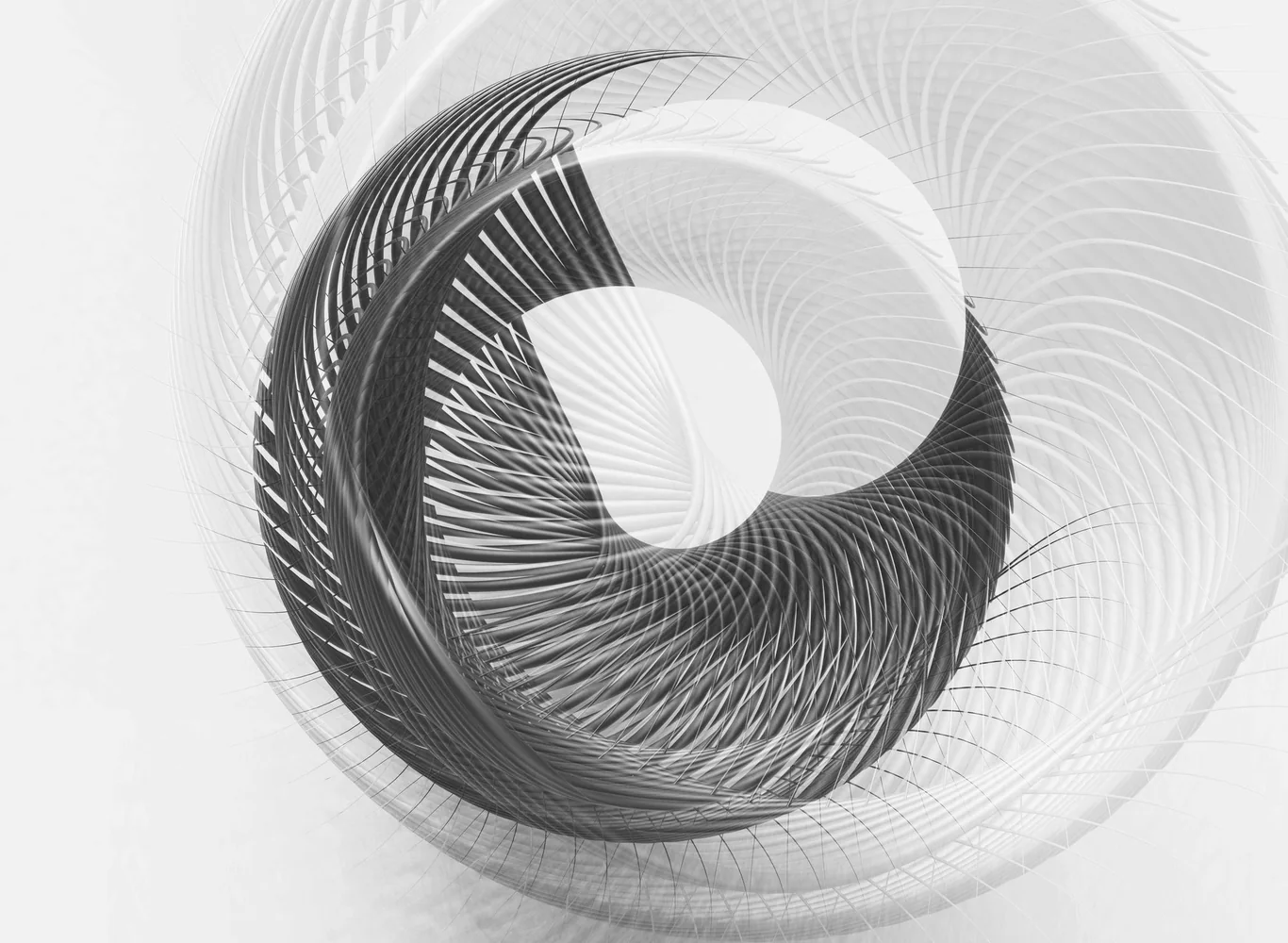
Mathematical Spirals: One Family, Several Growth Laws

1. Introduction

All spirals look alike at first glance: a curve that winds around a center while gradually moving away from it. Yet the way the radius grows with the angle defines mathematically distinct families, with radically different geometric properties and applications.

In polar coordinates, a spiral is defined by a relation $r=f(\theta)$ . The nature of this function — linear, exponential, square root, inverse — determines the entire behavior of the curve.

2. The Archimedean Spiral

The Archimedean spiral is defined by $r=a\theta$ , where a is a positive constant. The radius grows linearly with the angle: each full turn adds exactly the same distance to the radius. The coils are therefore equidistant.

r=a\theta

(Archimède)

Archimedes’ constant addition. The gold line compares two radii separated by one full turn: their difference always remains 2πa. This is the constant addition described by the formula.

This constant-spacing property makes it useful in clockwork mechanisms, flat springs, vinyl records and read heads. It also models the unwinding of a roll of paper or fabric.

3. The Logarithmic Spiral

The logarithmic spiral is defined by $r=ae^{b\theta}$ , where a and b are constants. The radius grows exponentially with the angle. Its most remarkable property is self-similarity: enlarged or reduced, it superimposes on itself. The angle between the tangent and the radius vector is constant, earning it the name equiangular spiral.

r = ae^{bθ}

(Logarithmique)

Logarithmic multiplication. The two blue radii point in the same direction one turn apart. Here, the measurement is not a fixed difference but a constant ratio, which explains self-similarity.

It appears in nautilus shells, galaxy arms, the flight paths of insects toward a light source, and phyllotaxis patterns. Jacob Bernoulli, fascinated by its properties, asked that it be engraved on his tombstone with the motto "Eadem mutata resurgo" (I shall arise the same, though changed).

4. Fermat's Spiral

Fermat's spiral is defined by $r^2=a^2\theta$ , i.e. $r=a\sqrt\theta$ . The radius grows as the square root of the angle. Unlike the previous two, it has two symmetric branches (for θ > 0 and θ < 0) and the coils tighten toward the outside.

r^2=a^2\theta,\quad\text{therefore }r=a\sqrt\theta

(Fermat)

Fermat’s two branches. The two colors show the two symmetric branches. The formula does not move the radius at the same rate as Archimedes’ law: multiplying r requires a larger increase in θ.

This is the spiral that best describes the arrangement of seeds in a sunflower or the scales of a pine cone, where the golden angle generates an optimal density distribution. It is also used in the design of certain turbines and heat exchangers.

5. The Hyperbolic Spiral

The hyperbolic spiral is defined by $r=\frac a\theta$ . The radius decreases as the angle increases: the curve winds toward the center without ever reaching it, and extends to infinity as θ approaches zero. It is the inverse of the Archimedean spiral in a precise sense.

r=\frac{a}{\theta}

(Hyperbolique)

Hyperbolic tightening. The arrow follows increasing θ: the radius decreases and the curve tightens. The central point is a geometric limit, not a destination that is reached.

It appears in certain optics problems and in modeling particle trajectories in force fields inversely proportional to distance.

6. Comparing the Families

Archimedean ( $r=a\theta$ ): equidistant coils, linear growth
Logarithmic ( $r=ae^{b\theta}$ ): self-similar, constant angle, exponential growth
Fermat ( $r=a\sqrt\theta$ ): two branches, increasing density outward
Hyperbolic ( $r=\frac a\theta$ ): decreasing radius, asymptote at origin

These four families are not exhaustive. There are also the Cotes spiral, the lituus, the Poinsot spiral and many parametric variants. But these four cover the vast majority of spirals encountered in science and engineering.

7. Conclusion

Classifying spirals by their radial growth law reveals that their visual similarity hides fundamentally different mechanisms. Identifying which spiral is present in a natural phenomenon or technical system is an essential step before any modeling.

The relation to the site’s thesis is precise: classifying spirals by their radial law may share geometry, dynamics, or representation with another family of phenomena, but these levels are not identical. Comparison becomes scientific when it names the proposed shared mechanism, the variables that differ, and the test that could distinguish them.

Approaching the phenomenon without confusing image and mechanism

The concrete starting point is classifying spirals by their radial law. Visible shape is not enough: coil spacing, tangent angle, and radial growth rate are different observables. An Archimedean spiral advances by addition, a logarithmic spiral by multiplication, and Fermat’s spiral by a square-root law. This difference in mechanism is the actual mathematical object. This first distinction matters because a winding form can be a trajectory, a structure, a projection, or simply a graphical convention.

The model that makes comparison testable

The polar representation $r=f(\theta)$ cleanly separates angle from distance to the center. Differentiating r gives radial change per unit angle; comparing r(θ + 2π) with r(θ) measures one-turn growth. This prevents us from calling every apparently regular curve “logarithmic.” ^[1] The model is not the object: it is a description whose assumptions must remain visible.

r=f(\theta)

(coordonnées polaires)

Reading a polar law. This sketch draws only one point P. θ fixes its direction; f(θ) fixes its radius. Varying θ produces the trajectory without confusing the angle, the distance, and the final curve.

Figure 1. Conceptual diagram: two polar laws can produce neighboring wound forms; the curves are not data.

From Continuous to Discrete: Measuring Turn by Turn

An equation describes a continuous curve, but a real measurement almost always arrives as separate points: a photograph, a set of coordinates, or a position recorded every ten degrees. Discrete mathematics provides a simple bridge between the ideal drawing and the observed object. Choose an angular step Δθ, then record each position in the order in which it is measured.

\theta_n=\theta_0+n\Delta\theta\ ;\ r_n=f(\theta_n)

(échantillonnage discret / discrete sampling)

n is an integer: 0, 1, 2, 3… The formula becomes an ordered sequence of measurements. These values can then be compared with Archimedean, logarithmic, Fermat, or hyperbolic laws instead of choosing the most convincing shape by eye.

Moving from curve to measurements. Each point n is a concrete observation. Their order carries the motion or construction; the blue curve remains the hypothesis that the measurements allow us to test.

An example, then its counter-example

The same drawing may describe a trajectory, a shell edge, or a geometric construction without retaining the same interpretation. In a construction, the equation directly causes the form. In a natural object, it may only be a local fit among biological or mechanical parameters. ^[2] The counter-example is as instructive as the example: it shows which variable is missing when moving from one domain to another.

What can actually be measured

To test a family, measure points and compare residuals with several models instead of choosing the most visually pleasing curve. A good comparison also reports uncertainty and the angular range over which the model remains valid. The spiral then becomes a quantifiable hypothesis rather than a label. A quantitative figure must distinguish published data, theoretical calculation, simulation, and conceptual diagram.

Decomposing variables instead of following the silhouette

To understand classifying spirals by their radial law, separate at least the variable that rotates, the one that changes scale, and the one that transports information or matter. Visible shape is not enough: coil spacing, tangent angle, and radial growth rate are different observables. An Archimedean spiral advances by addition, a logarithmic spiral by multiplication, and Fermat’s spiral by a square-root law. This difference in mechanism is the actual mathematical object. A global form can remain stable while its components are replaced; conversely, a trajectory can change shape without a new local mechanism.

The counter-example that protects the reasoning

The methodological lesson for Spirals Everywhere is clear: geometric resemblance may signal a shared constraint, but it does not demonstrate a shared origin. Here the convergence is among mathematical descriptions; it does not turn biological growth, a vortex, and an abstract curve into one phenomenon. We therefore cannot conclude from an image alone. We must ask which observation would falsify the hypothesis, then keep negative results in the comparison. This discipline is especially important when several models produce a similar outline.

A reproducible method

To test a family, measure points and compare residuals with several models instead of choosing the most visually pleasing curve. A good comparison also reports uncertainty and the angular range over which the model remains valid. The spiral then becomes a quantifiable hypothesis rather than a label. To make the result checkable, preserve parameters, units, resolution, initial conditions, and calculation method. An interactive visualization should also provide a readable initial state and a reset control; otherwise readers see an output without understanding its dependencies.

Open questions

The model explains the polar representation $r=f(\theta)$ cleanly separates angle from distance to the center. differentiating r gives radial change per unit angle; comparing r(θ + 2π) with r(θ) measures one-turn growth. this prevents us from calling every apparently regular curve “logarithmic.” ^[1] but does not answer questions at every scale. We still need to determine how initial conditions, perturbations, and system boundaries alter the pattern. This is where research begins: not by adding an analogy, but by formulating a prediction that could be measured.

Limits and scope of the analogy

Where the spiral is — and where it is not

References

[1]
Archimède. (-225). Sur les spirales. Traité mathématique
[2]
Bernoulli, Jakob. (1691). Spira mirabilis. Acta Eruditorum