Cardiac Spiral Waves: How Electrical Reentry Sustains Arrhythmia

1. Introduction

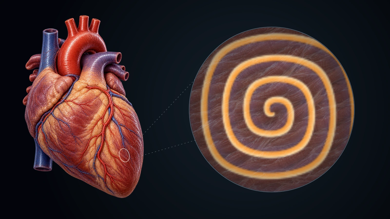
Every heartbeat results from an electrical wave that propagates in an orderly fashion through the myocardium, triggering the synchronized muscular contraction that propels blood. This wave originates in the sinoatrial node, traverses the atria, crosses the atrioventricular node, and then invades the ventricles within a few tens of milliseconds. When this orderly propagation is disrupted, a wave can fold back on itself and rotate indefinitely: this is reentry. Reentry is the primary cause of ventricular tachycardias and fibrillation — potentially fatal arrhythmias that constitute the leading cause of sudden cardiac death in industrialized countries.

The geometry of these reentrant waves is that of a spiral. Since the pioneering work of Wiener and Rosenblueth (1946) ^[1] and Winfree's experiments on chemical excitable media (1972) ^[2], followed by the numerical simulations of Panfilov and Holden (1990) ^[3], it has been established that cardiac tissue behaves as a two-dimensional (or three-dimensional) excitable medium in which spiral waves can form, anchor on anatomical heterogeneities, drift, fragment, and generate electrical turbulence. Understanding the physics of these spirals has become a major challenge in computational cardiology.

2. Cardiac Tissue as an Excitable Medium

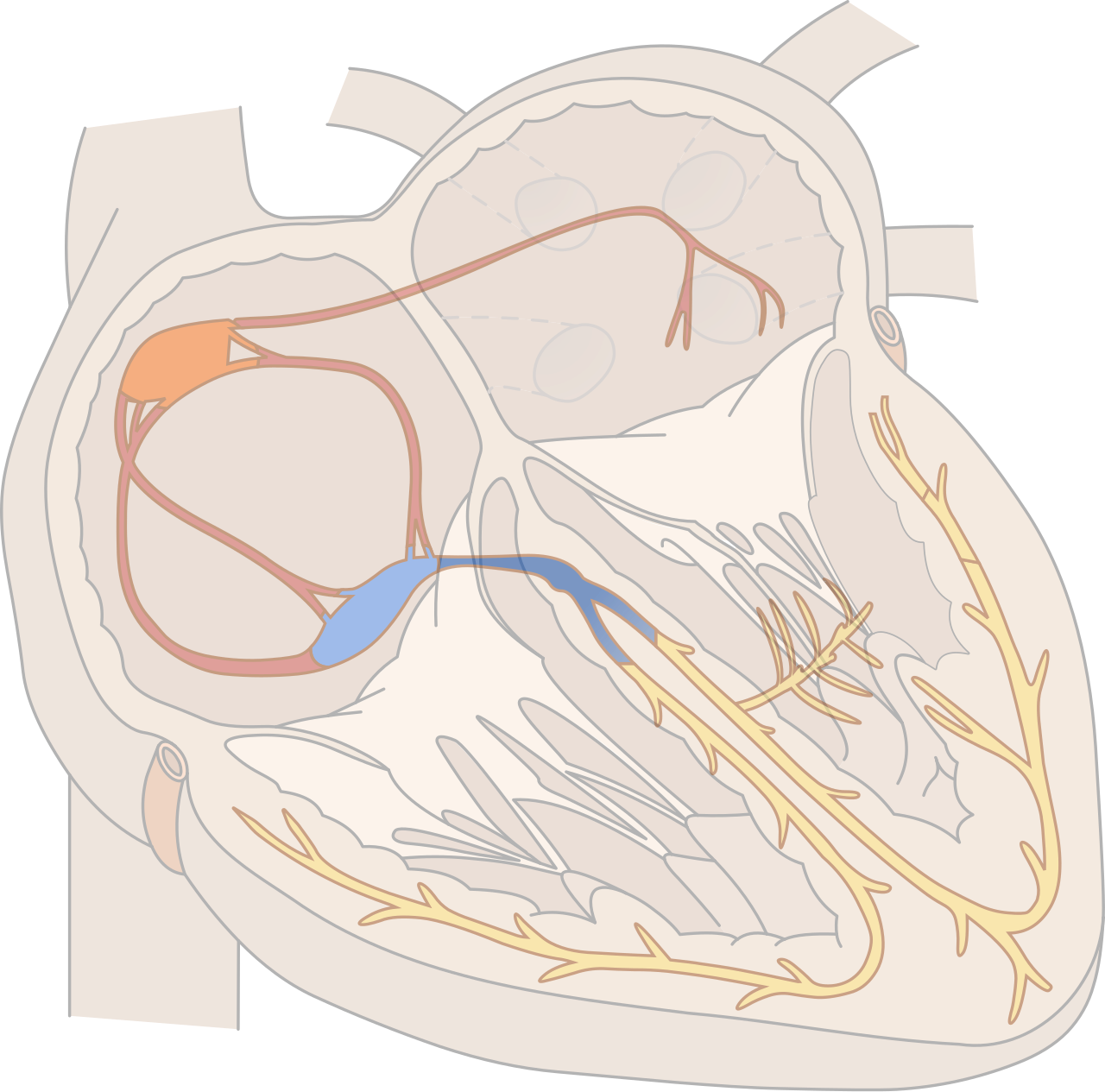
An excitable medium is a system with three fundamental properties: (i) a stable resting state, (ii) an all-or-nothing response to a perturbation exceeding a threshold, and (iii) a refractory period during which the medium cannot be re-excited. The myocardium fulfills all three conditions. Each cardiomyocyte is electrically coupled to its neighbors through gap junctions (connexins 40, 43, 45), forming a functional syncytium. Propagation of the depolarizing wave is driven by transmembrane ionic currents: the fast sodium current I_Na (depolarization), the slow calcium current I_CaL (plateau), and the potassium current I_K (repolarization).

The longitudinal conduction velocity in ventricular myocardium is approximately 0.5–1 m/s, and the transverse velocity is 3 to 5 times lower due to the anisotropy of muscle fibers. This anisotropy plays a crucial role in the formation and stability of spirals. The electrical wavelength λ = v × ARP (where v is the conduction velocity and ARP the absolute refractory period duration) determines the minimum size of a reentry circuit. For the human ventricle, λ ≈ 20–30 cm, meaning that reentry is only possible if the circuit is large enough or if the wavelength is reduced by ischemia or a drug.

3. The FitzHugh-Nagumo Model

The FitzHugh-Nagumo (FHN) model is the canonical mathematical reduction of an excitable medium. Originally proposed by FitzHugh (1961) ^[4] as a simplification of the Hodgkin-Huxley model, it describes the dynamics of a fast variable u (analogous to membrane potential) and a slow variable v (recovery variable, analogous to channel inactivation):

D: diffusion coefficient (spatial coupling); α: excitation threshold (0 < α < 1); ε ≪ 1: timescale separation; γ: recovery parameter; I_ext: external current.

In this model, the nullcline of u (∂u/∂t = 0 without diffusion) is an N-shaped cubic, and the nullcline of v is a straight line. Their unique intersection defines the stable fixed point (resting state). When u exceeds threshold α, the system makes a rapid excursion to the upper branch of the cubic (depolarization), then returns slowly (repolarization) via the lower branch. The refractory period corresponds to the time during which v is still elevated and prevents re-excitation.

In two dimensions, with the diffusion term D∇²u, the FHN model supports plane waves, circular (target) waves, and above all spiral waves. The spiral rotates around a rotation core (the "rotor") where u and v oscillate periodically. The rotation frequency of the spiral is higher than the natural frequency of the tissue, which explains why reentry takes control of the cardiac rhythm.

4. Spiral Waves and Reentry

A spiral wave in cardiac tissue is a depolarization wave that rotates around a phase-singular core. This core is a point (in 2D) or a filament (in 3D) around which all phases of the excitation cycle coexist simultaneously. Winfree (1987) ^[5] showed that this singular point is topologically inevitable: if a wave is broken (by a heterogeneity, localized ischemia, or a premature stimulus), its free ends necessarily curl into a spiral.

The classical mechanism for spiral creation is the S1-S2 protocol: a first stimulus S1 creates a plane wave; a second stimulus S2, applied during the refractory tail of S1, creates a wave whose one end is blocked (tissue still refractory) and whose other end propagates freely. This free end curls into a spiral. This mechanism was demonstrated experimentally by Davidenko et al. (1992) ^[6] on slices of canine ventricular myocardium using optical mapping with voltage-sensitive fluorescent dyes.

The shape of the cardiac spiral is an Archimedean spiral in simple models, but in realistic ionic models it more closely resembles a logarithmic spiral whose pitch varies with distance from the core. The rotation speed Ω and the core radius r₀ are determined by the local properties of the tissue (conduction velocity, action potential duration, slope of the restitution curve).

λ: electrical wavelength; v: conduction velocity; ARP: absolute refractory period duration; L_circuit: length of the anatomical or functional circuit.

5. From Tachycardia to Fibrillation

A stable, solitary spiral produces monomorphic ventricular tachycardia: the ventricle is activated at the rotation frequency of the spiral (typically 5–10 Hz, i.e., 300–600 bpm), well above the normal sinus frequency (1–2 Hz). Tachycardia is hemodynamically poorly tolerated because the high frequency reduces ventricular filling time and therefore cardiac output.

The transition to ventricular fibrillation corresponds to the fragmentation of the spiral into multiple daughter spirals, creating electrical turbulence. This phenomenon is linked to the instability of the spiral, itself governed by the action potential restitution curve. Karma (1993) ^[7] showed analytically that the spiral becomes unstable when the slope of the restitution curve exceeds 1:

APD: action potential duration; DI: diastolic interval (recovery time between two successive action potentials).

When the restitution slope exceeds 1, a slight variation in the diastolic interval is amplified at each cycle, producing an alternation of long and short action potentials (electrical alternans). This spatial alternation creates repolarization heterogeneities that fragment the wavefront into multiple independent spirals. Ventricular fibrillation is thus a state of spatiotemporal turbulence in an excitable medium.

6. Anchoring, Drift and Turbulence

In homogeneous tissue, the core of a spiral can drift slowly (translational motion of the rotor) or remain fixed. In the presence of anatomical heterogeneities (infarct scars, fibrotic zones, valvular orifices), the spiral can anchor to these obstacles. Anchoring stabilizes the spiral and makes tachycardia persistent. Panfilov and Vasiev (1995) ^[8] showed that the spiral preferentially anchors to obstacles whose size is comparable to the core radius r₀.

The drift of a free spiral in a slightly inhomogeneous medium can be described by equations of motion for the core. In the presence of a parameter gradient (for example a gradient of action potential duration due to ischemia), the spiral drifts perpendicular to the gradient (Doppler drift) and parallel to the gradient (gradient drift). These two drift components were calculated by Biktashev and Holden (1995) ^[9] using perturbation theory and the spiral response functions.

In three dimensions, the analogue of the spiral is a scroll wave, whose core is a filament. This filament can be straight, curved, or knotted. The dynamics of the filament are governed by curvature-tension equations: a curved filament contracts (positive tension) or extends (negative tension) depending on the medium parameters. Negative filament tension leads to a Winfree-Strogatz instability that fragments the scroll wave into many entangled filaments, producing the three-dimensional electrical turbulence observed in ventricular fibrillation.

7. Realistic Ionic Models

Beyond the FHN model, realistic ionic models have been developed to faithfully reproduce the human cardiac action potential. The Luo-Rudy model (1991, 1994) ^{[10] [11]} describes ventricular ionic currents in guinea pig with quantitative accuracy. The Ten Tusscher and Panfilov model (2006) ^[12] is the reference model for the human ventricle; it comprises 19 state variables and 12 distinct ionic currents.

These models are coupled to diffusion equations to simulate propagation in realistic cardiac geometries reconstructed by MRI. Simulating a complete human ventricle at cellular resolution (~10⁸ nodes) requires massive computational resources (supercomputers). Multi-scale approaches (cable models, finite elements, fictitious domain methods) allow reducing the computational cost while preserving the accuracy of clinical predictions.

C_m: membrane capacitance (~1 μF/cm²); V_m: membrane potential; I_ion: sum of transmembrane ionic currents; w: vector of channel gating variables; ρ_i: intracellular resistivity; σ_i: intracellular conductivity tensor (anisotropic).

8. Defibrillation and Spiral Control

Electrical defibrillation consists of applying an intense electrical shock (200–360 J for an external defibrillator) to simultaneously terminate all ongoing spirals. The mechanism is not simply a global tissue depolarization: Efimov et al. (1998) ^[13] showed by optical mapping that the shock creates virtual depolarization and hyperpolarization zones (virtual electrodes) that generate new waves, which can eliminate existing spirals if their timing is correct.

Alternative approaches to spiral control have been explored. Low-Energy Anti-fibrillation Pacing (LEAP) uses a sequence of low-amplitude shocks to progressively synchronize and eliminate spirals ^[14]. Feedback control uses real-time measurements of electrical activity to apply targeted stimulations that destabilize the rotor. These approaches aim to reduce defibrillation shock energy by 80 to 90%, thereby reducing tissue damage and pain.

Rotor mapping using endocavitary electrodes (FIRM system — Focal Impulse and Rotor Modulation) allows identifying spiral anchoring sites in atrial fibrillation and ablating them by radiofrequency ^[15]. This approach illustrates how the physical understanding of cardiac spirals translates directly into therapeutic strategies.

9. Conclusion

Cardiac spiral waves are one of the most dramatic and most studied manifestations of the physics of excitable media. Their existence results from a combination of universal properties — excitability, refractoriness, diffusive coupling — and anatomical particularities of the myocardium. The convergence between the theoretical physics of spirals (FHN models, perturbation theory, spatiotemporal turbulence) and clinical cardiology (optical mapping, radiofrequency ablation, low-energy defibrillation) is a remarkable example of how the mathematics of spirals illuminates vital phenomena.

The cardiac spiral is not a mathematical curiosity: it is a dynamic structure whose formation, stability, and destruction determine whether a heart beats or races. Understanding why and how an electrical wave re-enters cardiac tissue means understanding one of the most active frontiers between nonlinear physics and medicine.

References

- [1]Wiener, N. & Rosenblueth, A.. (1946). The mathematical formulation of the problem of conduction of impulses in a network of connected excitable elements, specifically in cardiac muscle. Archivos del Instituto de Cardiología de México, 16, p. 205–265
- [2]Winfree, A. T.. (1972). Spiral waves of chemical activity. Science, 175(4022), p. 634–636. DOI: 10.1126/science.175.4022.634
- [3]Panfilov, A. V. & Holden, A. V.. (1990). Self-generation of turbulent vortices by an excitable medium. Physics Letters A, 151(1–2), p. 23–26. DOI: 10.1016/0375-9601(90)90840-K
- [4]FitzHugh, R.. (1961). Impulses and physiological states in theoretical models of nerve membrane. Biophysical Journal, 1(6), p. 445–466. DOI: 10.1016/S0006-3495(61)86902-6
- [5]Winfree, A. T.. (1987). When Time Breaks Down: The Three-Dimensional Dynamics of Electrochemical Waves and Cardiac Arrhythmias. Princeton University Press
- [6]Davidenko, J. M., Pertsov, A. V., Salomonsz, R., Baxter, W. & Jalife, J.. (1992). Stationary and drifting spiral waves of excitation in isolated cardiac muscle. Nature, 355(6358), p. 349–351. DOI: 10.1038/355349a0
- [7]Karma, A.. (1993). Spiral breakup in model equations of action potential propagation in cardiac tissue. Physical Review Letters, 71(7), p. 1103–1106. DOI: 10.1103/PhysRevLett.71.1103
- [8]Panfilov, A. V. & Vasiev, B. N.. (1995). Vortex initiation in a heterogeneous excitable medium. Physica D: Nonlinear Phenomena, 82(3), p. 207–219. DOI: 10.1016/0167-2789(94)00222-K
- [9]Biktashev, V. N. & Holden, A. V.. (1995). Resonant drift of autowave vortices in two dimensions and the effects of boundaries and inhomogeneities. Chaos, Solitons & Fractals, 5(3–4), p. 575–622. DOI: 10.1016/0960-0779(93)E0044-C
- [10]Luo, C. H. & Rudy, Y.. (1991). A model of the ventricular cardiac action potential: depolarization, repolarization, and their interaction. Circulation Research, 68(6), p. 1501–1526. DOI: 10.1161/01.RES.68.6.1501
- [11]Luo, C. H. & Rudy, Y.. (1994). A dynamic model of the cardiac ventricular action potential. I. Simulations of ionic currents and concentration changes. Circulation Research, 74(6), p. 1071–1096. DOI: 10.1161/01.RES.74.6.1071
- [12]Ten Tusscher, K. H. W. J. & Panfilov, A. V.. (2006). Alternans and spiral breakup in a human ventricular tissue model. American Journal of Physiology — Heart and Circulatory Physiology, 291(3), p. H1088–H1100. DOI: 10.1152/ajpheart.00109.2006
- [13]Efimov, I. R., Cheng, Y., Van Wagoner, D. R., Mazgalev, T. & Tchou, P. J.. (1998). Virtual electrode-induced phase singularity: a basic mechanism of defibrillation failure. Circulation Research, 82(8), p. 918–925. DOI: 10.1161/01.RES.82.8.918
- [14]Luther, S., Fenton, F. H., Kornreich, B. G., Squires, A., Bittihn, P., Hornung, D., Zabel, M., Flanders, J., Gladuli, A., Campoy, L., Cherry, E. M., Luther, G., Hasenfuss, G., Krinsky, V. I., Pumir, A., Gilmour, R. F. & Bodenschatz, E.. (2011). Low-energy control of electrical turbulence in the heart. Nature, 475(7355), p. 235–239. DOI: 10.1038/nature10216
- [15]Narayan, S. M., Krummen, D. E., Shivkumar, K., Clopton, P., Rappel, W. J. & Miller, J. M.. (2012). Treatment of atrial fibrillation by the ablation of localized sources: CONFIRM (Conventional Ablation for Atrial Fibrillation With or Without Focal Impulse and Rotor Modulation) trial. Journal of the American College of Cardiology, 60(7), p. 628–636. DOI: 10.1016/j.jacc.2012.05.022