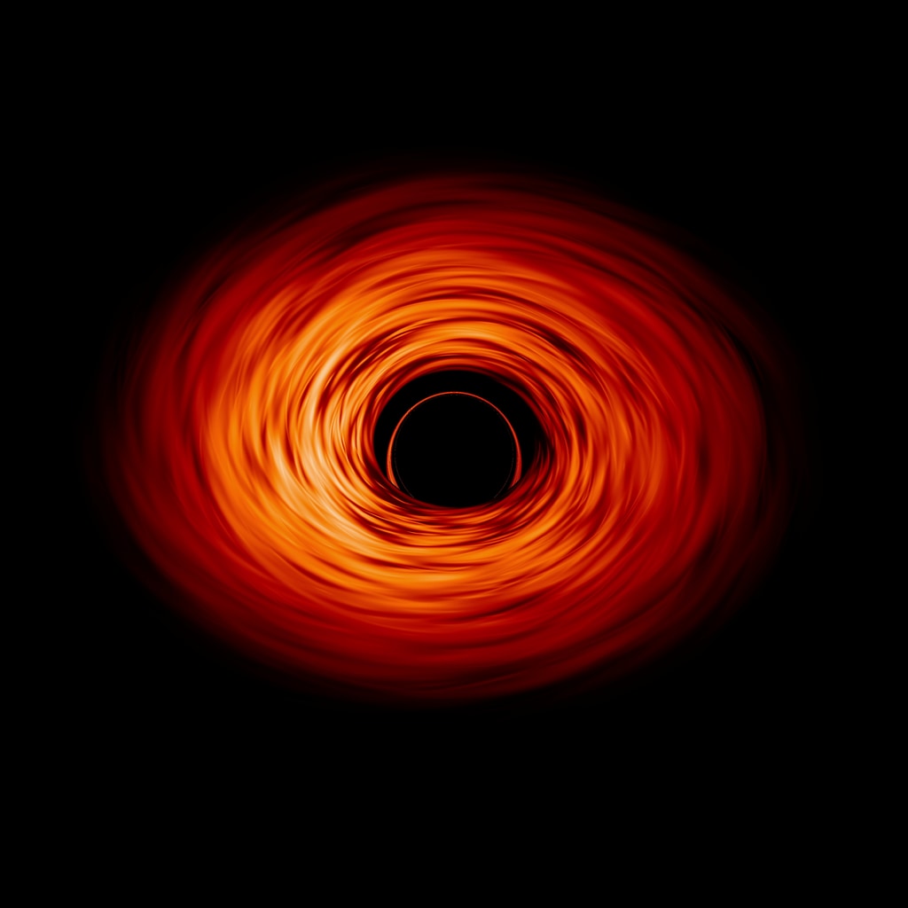
Dossier dated 6 November 2026. The study appeared online on 4 November and in the 6 November issue of Physical Review Letters. The NASA image shows an astronomical black-hole simulation, not the atomic experiment discussed here.
1. Build a cavity without moving a mirror at light speed
An ordinary Fabry–Pérot cavity traps light between two mirrors. Mimicking some horizon kinematics might suggest accelerating one mirror to an extreme speed, which is not an experimentally realistic route. Tanlimco and colleagues reverse the problem: they study a matter wave of ultracold lithium atoms confined between two sheets of light and periodically translate one barrier. The optical cavity becomes a model for organizing atomic-wave trajectories. [1]
The setup begins with a Bose–Einstein condensate of lithium-7 transferred into the second excited band of an optical lattice. Two repulsive light barriers then form a cavity about 681 μm long; an acousto-optic deflector periodically moves one barrier. Light therefore modulates the cavity length while the atoms provide the confined wave. The setup exchanges the usual roles: the wave is matter and the mirrors are made of light. No solid mirror is accelerated; an optical boundary is positioned with precision. [1]
The theoretical problem begins with a cavity whose length changes periodically. In a description sampled once per cycle, light trajectories can concentrate exponentially around particular space–time orbits. Stable and unstable fixed points of that map play roles analogous to white- and black-hole horizons. The obstacle was not drawing such trajectories but moving a massive mirror with the required effective accelerations. Here both the wave and boundary can be controlled at the atomic scale. [1]
2. What plays the role of light?
In the regime studied, the atomic-wave dispersion is quasi-relativistic over the relevant range: its group velocity can approach a characteristic limit of the system. The light sheets form reflecting boundaries, and one moves at a speed comparable to the wave. This speed remains below one metre per second. It is an analogy of dynamics and propagation: atoms do not become photons, and the laboratory does not create a black hole’s gravitational field. [1]
The choice of the lattice’s second band is crucial. Over a narrow range, its energy–quasimomentum relation is almost linear: its slope defines the atomic-envelope group velocity v_g and plays the role of an effective limiting speed. The authors set quasimomentum near this linear segment; the speed remains below 1 m/s. This reproduces the kinematic relations needed for the analogy at a very low laboratory speed. If atoms move too far from this range, band curvature changes their velocity and the photon analogy degrades. [1]
The resonance is not arbitrary: it depends on mean length L₀ and group velocity from the atomic band. In this cavity, fitting the trajectory without modulation gives Ω₀ = 95.1(5) Hz. This identifies the fundamental regime and allows comparison with drives at 95.5 Hz and then 191 Hz. The parenthetical digits express the authors’ uncertainty in the last reported figures. [1]
Dispersion relates a wave’s frequency to its wave number; its slope gives group velocity, the speed at which the pulse envelope travels. In the operating range, this relation is sufficiently similar to relativistic dispersion for a boundary moving at a comparable speed to reflect the wave. The atoms travel below one metre per second: the resemblance concerns kinematic equations at the chosen scale, not an absolute speed near light speed. [1] [2]
This relativity is effective and limited to a parameter range. The relevant speed is that of the matter-wave envelope, not a photon’s microscopic speed. Likewise, the “boundary” is a light sheet shaping the potential experienced by atoms, not a membrane that truly separates regions of spacetime. The experiment exchanges the roles of light and matter to reproduce a class of kinematics; it does not recreate every property of an electromagnetic cavity or a gravitational field. [1] [2]
3. A moving boundary transforms the problem
Periodic translation strongly drives the cavity. Rather than measuring only a resonance frequency, the experiment tracks an atomic pulse and asks where it ends up after several cycles. When modulation is near the cavity resonance—around 100 Hz in the reported regime—the pulse is steered toward a stable fixed point from several tested initial positions. An unstable fixed point instead repels nearby trajectories. Localization develops over a few cycles; it is not instantaneous compression or a photographed horizon. [1]
This map summarizes the stroboscopic reasoning: ξ represents the pulse state, P its evolution over one modulation period and ξ* a fixed point that returns to the same state each period. If nearby initial states move toward ξ*, it is stable; if they move away, it is unstable. This language turns a set of trajectories into a testable stability question. The formula is an explanatory schematic of the return map, not raw data or the full equation of the atomic system. [1]
“Stroboscopic” is essential: the wave’s position is compared at the same modulation phase, cycle after cycle. The authors sample twelve initial phases separated by π/6, time-shift the measurements for comparison and repeat each three times. Over about 80 ms, initially out-of-phase trajectories converge near the predicted stable point and move away from the predicted unstable point. The emergent pattern is not inferred from a selected image; it is convergence in synchronized measurements tested against the Floquet map. [1]
A fixed point is not a spot that stands still in a single image. It is a pulse state that returns to itself after one drive period under the return map P. The map’s local slope distinguishes the cases: a perturbation contracts around a stable point and grows around an unstable one. The accompanying teaching figure shows this criterion in a normalized state space; it is not a digitization of laboratory data. In the optical analogy, stable and unstable trajectories define trapping or escape regions associated with horizons. [1]
4. Modulation frequency changes the number of attractors
The landscape depends on drive relative to resonance. At 95.5 Hz, near the measured 95.1 Hz fundamental, an initially diffuse population concentrates onto a stable trajectory within a few cycles. At 191 Hz, the authors observe two stable fixed trajectories separated in phase by π. They halve the modulation amplitude to keep maximum boundary speed comparable, so the number of attractors is changed without also doubling boundary speed. These structures are observed responses of the driven system, not decorations added to the images. [1]
5. Why atoms depart from the light-wave prediction
The analogy has a measurable limit. Matter-wave dispersion is not perfectly linear; its residual curvature changes trajectories relative to a prediction treating the wave as ideal light. The authors connect observed deviations to this curvature. This strengthens the platform’s value: an analogue simulator does not replace theory; it makes visible the assumptions and corrections a simple analogy would neglect. [1]
The slope of the dispersion relation sets group velocity; its curvature makes components of a pulse evolve differently. The moving barrier can transfer energy to the atoms and push them toward quasimomenta where their velocity is no longer resonant with the drive. Simulations reproduce broadening near the stable focus and show loss of population from the D band. The authors also observe faint additional fixed trajectories absent from the simplest photon model. They attribute these deviations to nonlinear dispersion and velocity changes when reflecting from a moving wall. The mismatch with the ideal analogy is therefore a physical result to explain, not a flaw to hide. [1]
6. Reverse the dynamics with a phase jump
A sudden phase shift of the drive can exchange stable and unstable fixed points and reverse the direction of motion. This provides a controlled time-reversal operation in the pulse’s effective dynamics. Here the term describes reversibility of evolution in this driven model; it does not mean the laboratory rewinds history or reverses cosmic time. The manipulation illustrates how phase and temporal protocol structure trajectories in a non-autonomous system. [1] [2]
In the demonstration, the researchers apply a π phase jump after four cycles. The point that attracted the pulse becomes repulsive, the sampled evolution reverses, and the wave returns toward its starting trajectory. The protocol shows controlled decompression in the Floquet map. “Time reversal” refers to this stroboscopic reversibility under a specific drive: the atoms do not travel backward in time, and the process does not reverse dissipation or every microscopic variable. [1]
7. The black-hole comparison: useful, but bounded
A moving boundary can create regions where the wave propagates differently relative to the boundary; this kinematics motivates horizon analogies. But this experiment does not detect Hawking radiation, form an astrophysical gravitational horizon or observe a black hole. The cover image is a NASA simulation used only as astronomical context: it depicts an accretion disk distorted by gravity, unrelated experimentally to the atomic cavity. [2] [3]
8. What the result opens for wave physics
The immediate result is a matter-wave cavity in a strongly driven regime, with pulse concentration, control over the number of attractors and phase-based reversal. It offers a platform to explore moving-boundary dynamics using slow, measurable atoms. Pulse compression and signal control are longer-term possibilities, not demonstrated device performance. Follow-up work must quantify losses, repeatability, waveform sensitivity and parameter range before promising applications.
9. What should be measured next
The useful next step is not to multiply astrophysical analogies but to map the cavity’s limits: how many cycles are needed to attract the pulse, what dispersion shifts its trajectory, and how robust are fixed points to loss and noise? Maps should be repeated across initial phases, frequencies and waveforms, with uncertainties in position and convergence time. This would show where the analogy is robust and where atomic microphysics dominates. These questions extend the experiment; they are not already answered by the published result. [1]
Ultrastrong driving also opens a comparison across platforms. The authors suggest related dynamics could be implemented in electro-optic materials, where optical boundaries and pulses could be modulated differently. Pulse generation or compression is a possible application, but efficiency, stability, control range and advantage over existing optical techniques still need demonstration. The established contribution for now is an atomic platform that realizes and characterizes a regime previously difficult to access. [1]
References
- [1]Jeremy L. Tanlimco, Eber Nolasco-Martinez, Xiao Chai, S. Nicole Halawani, Eric Zhu, Ivar Martin et David M. Weld. (2026). Matter-Wave Fabry-Pérot Cavity in the Ultrastrong Driving Regime. Physical Review Letters, 137, p. 193404. DOI: 10.1103/44mq-jfp1. https://journals.aps.org/prl/abstract/10.1103/44mq-jfp1 — Primary research article; published online 4 November 2026, issue dated 6 November.
- [2]APS Physics. (2026). Atomic Wave Simulates Black Hole Properties. Physics Magazine. https://physics.aps.org/articles/v19/149 — Research overview published by the society’s magazine.
- [3]Jeremy Schnittman. (2019). Black Hole Accretion Disk Visualization. NASA Goddard Space Flight Center Scientific Visualization Studio. https://svs.gsfc.nasa.gov/13326/ — Astronomical simulation used as contextual imagery, distinct from the atomic experiment.